(See handout no.7; chapter 11)
The balance of payments is composed of the current account and the capital account, plus the monetary account (changes in reserve assets) which is really a settlement account of the above two.
Japan's Balance of Payments (Bank of Japan data, in trillions of yen)
| 2001 | 2002 | 2003 | 2004 | 2005P | Remark | ||
| Current account | 10.628 | 14.249 | 15.767 | 18.618 | 18.048 | ||
| of which | Goods (="trade balance") | 8.521 | 11.728 | 12.298 | 13.902 | 10.350 | |
| Services | -5.315 | -5.163 | -3.904 | -3.706 | -2.748 | ||
| Factor income | 8.390 | 8.279 | 8.281 | 9.273 | 11.360 | ||
| Transfer | -0.968 | -0.595 | -0.870 | -0.851 | -0.914 | Minus means net donation | |
| Capital account | -6.587 | -7.979 | 7.734 | 1.737 | -13.958 | ||
| of which | Foreign direct investment | -4.068 | -2.778 | -2.619 | -2.503 | -4.732 | Minus means net outflow |
| Other (loans, securities, deposits, etc) | -2.519 | -5.201 | 23.717 | 4.240 | -9.226 | Minus means net outflow | |
| Changes in reserve assets | -4.936 | -5.797 | -21.529 | -17.268 | -2.456 | Minus means increase | |
| (Memorandum) GDP | 501.280 | 497.532 | 501.647 | 505.186 | -- | ||
Note: Due to errors and omissions, numbers may not add up exactly. Classification systems differ from one country to another, and from one international organization to another.
Current account: payments related to current economic activities such as output, consumption, investment, employment, use of capital, etc. It is the sum of trade in goods and services, factor payments across countries (wage, interest, rent, dividend), and unilateral transfers (ODA grants, workers remittances, gifts, etc).
Capital account: payments related to transferring purchasing power from present to future, or vice versa, without a direct link with today's output, consumption, etc. These are normally called financial investments, or lending and borrowing (including repayments). Both official and commercial loans, long-term and short-term, are recorded here (including ODA loans). Implementation of FDI is also included in the capital account. Additionally, if FDI firms import machines and parts to start operation, such imports are recorded in the current account.
Current account + Capital account is called the Overall balance. This is the sum of all autonomous transactions (both private and official), which may be positive or negative.
Monetary account: the use of "money" to settle the sum of the two accounts above. If the overall balance is positive (total receipts > total payments), international money accumulates, and vice versa. Actually, this is recorded as an increase or decrease of net foreign assets of the monetary institutions collectively (including the central bank and commercial banks).
Our question in this lecture is: how is the current account determined?
There are four basic models.
(1) Inter-temporal optimization model
(2) Absorption approach
(3) Saving-investment balance approach
(4) Elasticities approach
We will discuss them in turn. The second and the third model can be regarded as logically equivalent. If we combine them, we have three basic models. Ideally and theoretically, these different models should be mutually consistent. But actually, it is difficult to reconcile them and practical policy implications often differ significantly from one model to another, as we will see below.
This is a microeconomics-based approach. In this model, the current account is the result of people's collective optimization behavior under the inter-temporal budget constraint. In a nutshell, the current account is determined by spontaneous lending and borrowing.
A current account surplus means that a country is producing more than it spends. It exports more than it imports, so the country is a net lender to the world. Conversely, a current account deficit means that spending exceeds production, imports are greater than exports, and the country is borrowing from the world.
This model basically says that these lendings and borrowings are optimal. Unless there is a market failure or distortive official intervention, it is assumed that the collective behavior of the nation is rational.
If people are rational and information is (reasonably) perfect, and if capital mobility is guaranteed, then production choice and consumption choice across time (today and tomorrow) can be made separately. People lend or borrow in order to smooth consumption. This can be easily depicted by an elementary microeconomics diagram featuring preference and a budget line. In this case, the relative price between today's goods and tomorrow's goods is the interest rate (more precisely, one plus interest rate). The model can be worked out with or without investment, with or without infinite periods, etc. It is very easily handled and mathematically neat.
The greatest strength (as well as the weakness) of this model is its theoretical beauty. It can also produce the balance-of-payments cycle theory (a young developing country first borrows, then lends and accumulate foreign assets as it reaches maturity, then lives out of its earned interest in the old age, etc.). But we can ask: are people really rational (remember the Asian crisis)? Especially, do governments really behave rationally and with a long-term vision?
The famous textbook that expounds this approach (even to a quite advanced level) is Obstfeld-Rogoff listed in the reference section below.
This is a macroeconomics-oriented approach. That means the model is formulated without direct reference to people's optimizing behavior. It is based on a few simple macroeconomic identities. Its strength is simplicity and practicality. Its weakness is the lack of deep theoretical foundation. But maybe this approach is more useful for looking at the real situation of your country. (It can be said that the inter-temporal optimization model above is a much stronger model than this, because it not only satisfies obvious identities but also assumes optimization.)
Start with the well-known national income identity:
Y = C + I + G + X - M
(Y: income C: private consumption I: private investment G: government spending X: exports M: imports)
C + I + G is often called "domestic demand." But here, we use a more technical term "absorption" or "A." They are the same thing.
A = C + I + G (definition)
The current account CA is X - M (here, we ignore other items in the current account like ODA grants, factor income, etc).
CA = X - M (definition)
From above, we can easily see that
X - M = Y - A
or simply, CA = Y - A.
In words, the current account is an excess of a nation's production (=income Y) over absorption (=domestic demand or A). Y is what the country produces and A is what it spends (for consumption and investment) and the gap is CA.
A current account (CA) surplus (the situation depicted in the diagram above) means the country underspends its income (like Japan, China, Taiwan), and a CA deficit means it overspends its income (USA and many developing countries). Usually, the latter is the bigger problem for policy makers. If a country is experiencing a CA deficit, there are only two solutions according to this model: increase Y or decrease A.
Increasing Y is a supply-side problem. The IMF thinks that economic liberalization (free trade, privatization, deregulation, etc.) will unleash private sector dynamism and boost output. But this will take time, even if it is successful.
Decreasing A is a demand-side problem. Usually, it means austerity--tight budget and tight money. This is the most traditional IMF conditionality, which is supposed to work immediately as the policy is implemented.
So the classical IMF solution is: macroeconomic adjustment (with a painful but immediate effect) combined with economic liberalization (expanding the size of the economic pie in the long run).
As noted earlier, the saving-investment approach is very similar to the absorption approach, because it is based on one additional simple identity. It is simple, macroeconomics-oriented, and useful for discussing the reality.
Recall the previous national income identity on the expenditure side:
Y = C + I + G + X - M
To this, we add the national income identity on the disposal side (how people earn income and allocate it to different uses):
Y = C + S + T
(S: saving T: taxes)
This says that income is divided into consumption, saving and taxes. (Sequentially, maybe it is more reasonable to say, first we pay taxes, then spend, and save the remainder. Or maybe you save first? If we are rational, all these decisions should be simultaneously made.)
From these two identities, Y and C cancel out, and it is easy to see:
X - M = (S - I) + (T - G)
Remember, this is still an identity (which means it always holds, whether in equilibrium or non-equilibrium). The CA (= X - M) is identically equal to net private saving (S - I) plus net government saving (T - G). The current account is the net saving of the two sectors combined.
According to this view, a CA deficit means that either the private sector or the government (or both) has negative saving (called dissaving). In many cases, it is the government that overspends its budget. Or maybe both sectors are dissaving (i.e., suffer from savings shortage).
To reduce the CA deficit, there are only two ways. Increase net private saving or increase net government saving.
To increase net private saving (S - I), discouraging investment is generally undesirable (unless there is an investment bubble). The better solution is to encourage private saving. This can be done by various institutional adjustments to strengthen incentives to save and remove incentives to consume too much, in the the tax system, banking, housing, pension, social security and insurance, etc.
To increase net government saving (T - G), you must either increase tax revenue or cut spending. Usually, the IMF recommends both.
The elasticities approach is another, entirely different theory. It is easy to understand (and misunderstand) and appeals to laymen without the knowledge of economics. Also, many "top-class" economists take the elasticities approach as granted and any doubt cast on this theory is often severely criticized by them. But my feeling toward this approach is: it is misleading and must be handled with much care.
The strength of this approach is general appeal. Its weakness is that it captures only a small part of the situation. Technically, this is called "partial-equilibrium analysis" (that is, looking at the traded goods market only and ignoring the interaction of various markets in the entire economy; the alternative approach that looks at all markets is called "general equilibrium analysis").
It begins with the observation that CA is the gap between exports and imports. The quantities of imports (QM) and exports (QX) are determined as follows, respectively:
QM = f ( Y, EP*/P), f1>0, f2<0
QX = g ( Y*, EP*/P ), g1>0, g2>0
(E: nominal exchange rate P: domestic price P*: foreign price)
Quantities of exports and imports are each determined by two factors: (1) income (or "scale") variable, domestic or foreign; and (2) real exchange rate (=relative price). Here, f1, f2, g1, g2 are partial derivatives. For example, f1>0 means that if Y rises, QM is positively affected (i.e., also rises).
If we regard P as the export price and P* (or EP* in domestic currency) as the import price, we have:
CA = P QX - (EP*) QM
The current account is (price x quantity) of exports, minus (price x quantity) of imports.
In this model, if a country wishes to reduce a CA deficit, what should be done?
The answer is to depreciate the home currency (in our notation, a rise in E). At first, a rise in E will worsen the CA deficit. But later, as trade quantities QX and QM gradually respond to the relative price change, the initial negative effect is overcome and CA begins to improve (QX rises and QM falls). This pattern of initial worsening and later improvement is called the J-curve effect, because if CA is plotted against a horizontal time axis, it looks like an elongated and tilted letter J as below:
The big question is: do QX and QM respond sufficiently to offset the initial worsening caused by E? In other words, are the price elasticities of export and import quantities large enough? This is why this approach is called the elasticities approach (i.e., the result depends on the two elasticities).
Under the simplifying assumption that domestic and foreign prices do not change (no pass-through) after a depreciation, with initial trade balance, we can derive the condition for effective depreciation (the condition that a depreciation will improve CA, rather than worsen it). It is simply the following:
(Price elasticity of exports) + (Price elasticity of imports) > 1
Note that both elasticities are defined as positive (in absolute value). Sufficiently large elasticities here mean that their sum is greater than one. This is called the Marshall-Lerner condition. Marshall and Lerner were the economists who proposed this a long time ago. If we have other assumptions (like prices are not fixed, income changes, there is a nontradable good, initial trade is not balanced, etc), we can make this condition more complicated.
Almost all large-scale world econometric models contain equations for the quantities of exports and imports based on the elasticities approach. They additionally have equations for determining the export and import prices.
In the 1980s, many US economists (including Fred Bergsten and Paul Krugman) argued that a devaluation of the US dollar was effective in reducing the US current account deficit. They argued that Y and Y* influenced CA immediately, but a change in the real exchange rate (EP*/P) took about two years to influence trade flows. Using this logic, they urged Japan to (1) take an expansionary fiscal policy; and (2) appreciate the yen against the dollar, in order to reduce Japan's surplus with the US. (Additionally, US economists often demanded Japan to buy more American goods and sell less to America.)
But why do I say this approach is misleading? The main reason is that this is a partial-equilibrium analysis assuming all other things (key macro variables) remaining the same, even when E changes. But actually, "other things" may systematically shift when the currency is depreciated.
(1) Prices are often affected by the exchange rate (E => P, P*: this is called the pass-through effect). If prices adjust proportionally, there will be no change in the real exchange rate in the long run. This effect is particularly strong for a small open economy.(2) Output and business condition may be affected by depreciation or appreciation (E => Y, Y*). In Japan, output recession has often been observed after a sharp yen appreciation, offsetting the expected effect of exchange rate adjustment (recession tends to increase the trade surplus, rather than reduce it).
(3) Monetary policy must adjust (i.e., become more expansionary) if the exchange rate depreciation is to be engineered. But monetary expansion, namely a shift in the LM curve, will upset the whole macroeconomic balance and create domestic boom and inflation (in the case of depreciation) or recession and deflation (in the case of appreciation). This will also offset the intended effect.
So, the statement that "depreciation improves the current account" seems a bit too simplistic. Whether that will be true or not depends on the parameter configuration of each country, which in turn depends on the complex conditions that each country faces. For example, if the economy is small and open, pass-through should be substantial. These offsetting effects, when combined, may easily overwhelm the intended relative-price effect.
The monetary approach to the balance of payments is a theory under a fixed exchange rate regime. By contrast, the monetary approach to the exchange rate is its application to a floating exchange rate regime. As the names suggest, they argue that the demand and the supply of money is key. They were advocated by University of Chicago economists, including Harry G. Johnson, Michael Mussa, and Jacob Frankel (the latter two were former IMF chief economists).
The monetary approach to the balance of payments does not explain the current account. Rather, it is a theory of the overall balance, which is the mirror image of the monetary account (see above). It says that the overall balance, or net monetary inflow, of a country is determined by how fast the domestic money supply is growing relative to money demand. If monetary growth is faster than the growth of money demand, the country has an excess supply of money. Thus money flows out (=reserve loss) and the overall balance becomes negative. The situation of excess demand for money is just the opposite. Throughout, prices are assumed given at the world level under a fixed exchange rate. Money becomes endogenous under this situation. This idea was popular in the 1960s and the early 1970s.
On the other hand, the monetary approach to the exchange rate says that the floating exchange rate is determined by purchasing power parity (PPP). PPP in turn is determined by the money market equilibrium (money supply equals money demand) in each country. So the exchange rate is ultimately determined by M, Y and i of the two countries (and nothing else):
PPP: E = P/P*
Money market (domestic): M/P = L(Y, i) [solving for P, we have P = M/L(Y,i) ]
Money market (foreign): M*/P* = L*(Y*, i*) [solving for P*, we have P* = M*/L*(Y*,i*) ]
Inserting P and P* into the PPP equation, we have:
E = [M/L(Y,i)]/[M*/L*(Y*,i*)]
Both of these theories were advocated in the age of little private capital flows. Today, no one really uses them.
Let us ask the following question.
Assume international capital mobility. Under this, we can generally expect that the savings (S) and investment (I) will not necessarily be equal in each country (that is, we should normally observe S > I or S < I). This is because S and I are determined by different sets of variables.
Savings depend mainly on income. Additionally, they are affected by the development and stability of the financial sector, credibility of monetary policy, inflation and exchange rate expectations, pension and social security systems, housing markets, demography (especially the aging of the population), use of credit cards and electronic money, etc.Investment is a function of technology, business opportunity, expected returns and risks, existing capital stock, long-term capital market, bank loans, policy and legal investment environment, etc.
S and I are both affected by the interest rate. But with open financial markets and uncovered interest parity (lecture 4), the domestic interest rate will be determined internationally: it is equal to the global interest rate plus the exchange rate expectation (plus a risk premium). At that rate, there is no guarantee that domestic S and domestic I will be equal. Since motives of S and I are different, why should we expect them to be equal? If all countries optimize inter-temporarily, some should have excess savings and others should have excess investment. If S > I, the country will have a CA surplus. If S < I, there will be a CA deficit. And there should be little correlation between the movements of S and I in each country.
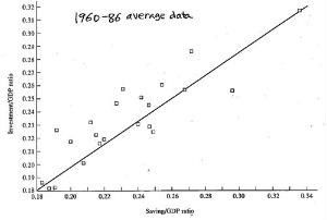
But when Martin Feldstein (a Harvard University professor) and Mr. Charles Horioka (his research assistant then; now he teaches at Osaka University) looked at cross-country data for 1960s and 70s, S and I were very positively correlated within each country. A high savings country also tended to have high investment, and vice versa. So we have S = I for each country, or nearly so.
| S-I correlation in 23 OECD countries 1960-86 average data |
S-I correlation within USA 1960 to 1990 |
 |
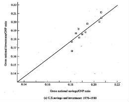 |
Source: Batiz-Batiz (sub-textbook), pp.271-272.
They were puzzled and wrote a paper in 1980 arguing something like this: "Maybe there is no true capital mobility. Financial markets are segmented internationally. That is why the S-I gap within each country is very small." This started a fairly animated debate. Other economists proposed alternative explanations for observing S = I, even under capital mobility.
The first alternative explanation was the "Ricardian Equivalence." (David Ricardo was a famous 19th century British economist. His idea was resurrected by Princeton Professor Robert Barro.) Remember one of the equations above,
CA = (S - I) + (T - G)
or CA is equal to the sum of net private saving and net government saving. Suppose the government increase its spending, G, without raising T. If people are rational and far-sighted, they will immediately understand that this public spending financed by government bond issuance will increase future tax burden (to repay government bonds, taxes must be increased). They will try to offset the expected lower disposable income in the future by saving more today. Therefore, as G rises, S also rises by the same amount (i.e., consumption, C, falls). CA is unchanged. What happened is a shift in the composition of today's spending (more G and less C) with no change in the total spending. Since any action by the government (T-G) is offset by the private sector (S-I), the national net saving does not change.
 |
|
 |
 |
|
| Martin Feldstein (1939-) | Charles Yuji Horioka (1956-) | David Ricardo (1772-1823) | Robert Barro (1944-) |
The second alternative explanation is quite the opposite. Tam Bayoumi (he and I were classmates at Stanford University) wrote a paper arguing that maybe it is the government that is offsetting private shocks. When (S-I) is upset because of investment boom (say), the government adjusts its fiscal balance (i.e., tightens the budget) to cool it. When (S-I) falls because of sudden pessimism (say), the government spends more. So again, CA is unaffected.
But why does the government want to do the offsetting? Because they care about the current account position as well as avoiding excessive business swings. Bayoumi shows that, when fiscal policies were not active during the Classical Gold Standard period, 1880-1913, S and I were less correlated. Only after the Keynesian fiscal policies were invented and became quite popular, in 1965-86 for example, the tendency for S = I has become apparent.
The third possible explanation is called home-currency preference. Even if capital is mobile, people prefer home currency or they have a "currency habitat." The private sector does not wish to accumulate foreign assets too much, so the net lending or borrowing is confined to near zero. (But central banks may be less worried about holding foreign currency. In Japan, China and Taiwan, the public sector accumulates huge amounts of foreign assets despite potential exchange risk.)
More recent data (1999) for OECD countries show that domestic savings and investment are beginning to be not-so-highly correlated--see below. As global capital mobility rises, countries are beginning to lend or borrow significantly as in the Classical Gold Standard period. After all, Feldstein and Horioka's puzzle may not be a puzzle at all; they probably used the data that were too early for testing capital mobility.
Savings and Investment in OECD Countries
(1999, in percent of GDP)
Since around the 1970s, Japan persistently had a trade surplus with the US, and the US persistently had a trade deficit with Japan. In recent decades, Japan had the largest trade surplus in the world and the US had the largest trade deficit in the world. The capital flow from Japan to the US was the largest bilateral capital flow in the world. [Again, we do not distinguish the current account and the trade balance since the difference was rather small and stable.]
At the same time, China is catching up very quickly with Japan as a supplier of savings to the United States. In the 21st century, China has emerged as the largest surplus country with the US, overtaking Japan. As a result, the US congress and trade negotiators are now more critical about China's export drive than Japan's. Notice that the Japan-US trade gap exhibits cyclical movements over several years while China's surplus increases smoothly without such cycles. Presumably, this is due to China's fixed exchange rate in comparison with Japanese yen's fluctuation. (In other words, the floating exchange rate can have cyclical impacts on the nation's current account but does not affect its long-term trend.)
Sources: US Bureau of Economic Analysis, US
Census Bureau.
A few remarks are in order about the Japan-US trade gap.
(1) Data confirm the Feldstein-Horioka observation, namely, the US savings and US investment were highly correlated over time (they moved in a similar way every year), and so were Japanese savings and investment. But this relation was tight only up to around 1982. After that, there was less S-I correlation within each country. Apparently, this reflects the capital account liberalization undertaken by Japan in 1980.
(2) The Japanese savings rate (public and private) was always higher than the US savings rate. Many economists (including Charles Horioka) advanced alternative theories to explain why the Japanese saved so much, including: (i) life-cycle saving hypothesis under the aging population; (ii) housing factors--mortgage interest payments are subsidized in the US while Japanese must put up a large down payment to buy a house; (iii) bequest motive--Japanese parents save a lot for children while Americans spend all their money and die; (iv) social welfare is more advanced in the US than Japan, so Americans don't have to save.
(3) According to the savings-investment balance approach,
X - M = (S - I) + (T - G),
the persistent US current-account deficit is due to (i) US government deficit, (T-G<0) ; (ii) US private saving shortage (S-I<0); or both. In the 1980s, the US had a huge fiscal deficit which was blamed for the equally large current-account deficit. But in the 1990s, the US fiscal balance improved dramatically, even to a big surplus, thanks to the sustained IT and stock market boom. But now, the boom has ended and the cost of war in Iraq must be paid. The US fiscal balance is back in the red again. All this while, US households continued to save very little. Low household saving is a common characteristic of Anglo-Saxon countries, including the US.
The Ministry of Finance data show that Japan had a net external asset position of $1.79 trillion (equivalent to 37% of GDP) at the end of 2004. Among this, 58% was held by the private sector and 42% by the public sector. The Bank of Japan's foreign reserves were $845 billion then (by May 2006, it rose slightly to $860 billion). Even though China is catching up fast, Japan is still the world's largest creditor country. And the US, although economically and militarily the strongest, is the world's largest debtor country.
This is an abnormal situation. Historically, the leader country which provides the international money tends to be also the largest creditor country, supplying capital to the rest of the world (as the UK did from the 19th to the early 20th century). But today's leader country (US) is importing massive capital from Japan, China, Taiwan, etc. to cover its domestic savings shortage. If the foreign debt burden becomes too large, the US can print greenbacks to repay the debt because the dollar is still accepted as an international currency. But that will risk a global inflation and the dollar's collapse. Japan, China, and other countries which hold large amounts of dollar assets will incur huge exchange losses. Who will make sure that this will not happen?
From the Japanese perspective, Japan is a fragile creditor because of the following reasons:
(1) Japan is not the largest or strongest economy in the world and, as a consequence, it cannot take the lead in global economic matters. Its economic diplomacy is often passive.
(2) Japan lends in USD, which means that it faces exchange risk each time the yen/dollar rate fluctuates. (The only exception is the ODA yen loans which are not subject to exchange risk, at least for Japan).
(3) Unlike the US or EU, Japan has no yen zone around it (East Asia is actually a dollar zone). Every movement of the yen/dollar rate impacts Japan directly, since it has no currency "buffer zone." Additionally, the economic relationship between Japan and the rest of East Asia is also affected by the yen/dollar rate fluctuation.
As a result, Japan (and East Asia) is vulnerable to exchange rate-driven macroeconomic and financial shocks to a much greater extent than the US or EU economy. In Japan, a high yen causes the loss of competitiveness, output recession, price deflation, instability in interest rates and their term structure, an exodus of Japanese FDI into the rest of East Asia, the balance-sheet problems of banks and corporations, etc. etc.
To avoid these shocks, Japan has tried to stabilize the yen/dollar exchange rate as well as promote the use of yen in East Asia (called the "internationalization of the yen"). [I am supportive of the first effort but not the second.] The general lesson seems to be that, if you are the largest creditor in the world but not very powerful in other aspects, the status of the top savings provider will bring you a lot of trouble and uncertainty and not much benefit.
The situation of being a vulnerable creditor country in a world where the dollar dominates is called conflicted virtue by Prof. Ronald McKinnon of Stanford University (McKinnon 2005--see below). For more, please see handout no.3 and the syndrome of the ever-higher yen in lecture 3.
<References>
Bayoumi, Tamim, "Saving-Investment Correlations," IMF Staff Papers 37:2, June 1990.Feldstein, Martin, and Charles Yuji Horioka, "Domestic Savings and International Capital Flows," Economic Journal, June 1980.
McKinnon, Ronald I., and Kenichi Ohno, Dollar and Yen: Resolving Economic Conflict between the United States and Japan, MIT Press, 1997 (Japanese translation, Nihon Keizai Shimbunsha, 1998).
McKinnon, Ronald I., Exchange Rates under the East Asian Dollar Standard: Living with Conflicted Virtue, MIT Press, 2005.
Obstfeld, Maurice, and Kenneth Rogoff, Foundations of International Macroeconomics, MIT Press, 1996.
